Background
In this mini-project, you will explore FiveThirtyEight’s Halloween Candy dataset.
We will use lots of ggplot some basic stats, correlation analysis and PCA to make sense of the landscape of US candy - something hopefully more relatable than the proteomics and transcriptomics work that we will use these methods on throughout the rest of the course.
Data Import
Our dataset is a CSV file so we use read.csv()
<- read.csv ("candy-data.txt" , row.names= 1 )head (candy)
             chocolate fruity caramel peanutyalmondy nougat crispedricewafer
100 Grand            1      0       1              0      0                1
3 Musketeers         1      0       0              0      1                0
One dime             0      0       0              0      0                0
One quarter          0      0       0              0      0                0
Air Heads            0      1       0              0      0                0
Almond Joy           1      0       0              1      0                0
             hard bar pluribus sugarpercent pricepercent winpercent
100 Grand       0   1        0        0.732        0.860   66.97173
3 Musketeers    0   1        0        0.604        0.511   67.60294
One dime        0   0        0        0.011        0.116   32.26109
One quarter     0   0        0        0.011        0.511   46.11650
Air Heads       0   0        0        0.906        0.511   52.34146
Almond Joy      0   1        0        0.465        0.767   50.34755
Q1. How many different candy types are in this dataset?
There are 85 in this dataset
Q2. How many fruity candy types are in the dataset?
38 fruity candy types.
Q3. What is your favorite candy (other than Twix) in the dataset and what is it’s winpercent value?
"Milky Way" , "winpercent" ]
Attaching package: 'dplyr'
The following objects are masked from 'package:stats':

    filter, lag
The following objects are masked from 'package:base':

    intersect, setdiff, setequal, union
|> filter (row.names (candy) == "Milky Way" ) |> select (winpercent)
          winpercent
Milky Way   73.09956
Q4. What is the winpercent value for “Kit Kat”?
"Kit Kat" , "winpercent" ]
Q5. What is the winpercent value for “Tootsie Roll Snack Bars”?
"Tootsie Roll Snack Bars" , "winpercent" ]
Q6. Is there any variable/column that looks to be on a different scale to the majority of the other columns in the dataset?
Yes! Winpercent seems to be out of 100, which is very different from other columns.
Q7. What do you think a zero and one represent for the candy$chocolate column?
 [1] 1 1 0 0 0 1 1 0 0 0 1 0 0 0 0 0 0 0 0 0 0 0 1 1 1 1 0 1 1 0 0 0 1 1 0 1 1 1
[39] 1 1 1 0 1 1 0 0 0 1 0 0 0 1 1 1 1 0 1 0 0 1 0 0 1 0 1 1 0 0 0 0 0 0 0 0 1 1
[77] 1 1 0 1 0 0 0 0 1
The 1 represents TRUE while the 0 represents FALSE.
Exploratory analysis
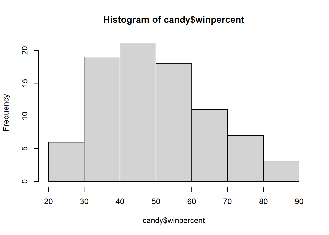
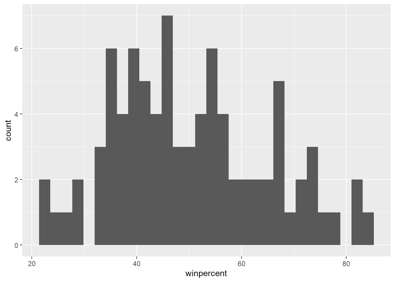
Q8. Plot a histogram of winpercent values.
library (ggplot2)ggplot (candy) + aes (winpercent, bins= 30 )+ geom_histogram ()
`stat_bin()` using `bins = 30`. Pick better value `binwidth`.
Q9. Is the distribution of winpercent values symmetrical?
No, it is skewed to the left.
Q10. Is the center of the distribution above or below 50%?
It is above 50%.
summary (candy$ winpercent)
   Min. 1st Qu.  Median    Mean 3rd Qu.    Max.
  22.45   39.14   47.83   50.32   59.86   84.18
Q11. On average is chocolate candy higher or lower ranked than fruit candy?
Find all chocolate candy
Get their winpercent values
Find the mean
Find all fruity candy
Get their winpercent values
Find the mean
Compare the two means
<- candy[candy$ chocolate == 1 , ]<- choc.candy$ winpercentmean (choc.win)
<- candy[candy$ fruity == 1 , ]<- fruity.candy$ winpercentmean (fruity.win)
Chocolate is higher ranked than fruity candy.
Q12. Is this difference statistically significant?
t.test (choc.win, fruity.win)
    Welch Two Sample t-test

data:  choc.win and fruity.win
t = 6.2582, df = 68.882, p-value = 2.871e-08
alternative hypothesis: true difference in means is not equal to 0
95 percent confidence interval:
 11.44563 22.15795
sample estimates:
mean of x mean of y
 60.92153  44.11974
Yes, they are statistically different cause p-value is less than 0.05.