Joseph's Site
My classwork for BIMM143
Class 13: RNASeq with DESeq2
Joseph Lo (PID: A18121493)
- Background
- Data Import
- Differential gene expression
- DESeq analysis
- Volcano Plot
- Adding some color annotation
- Save our results
- Add annotation data
- Save annotated results to a CSV file
- Pathway analysis
Background
Today we will perform an RNASeq analysis of the effects of a common steroid on airway cells.
In particular, dexamethasone (herafter just called “dex”) on different airway smooth muscle cell lines (ASM cells).
Data Import
We need two different inputs:
- countData: with genes in rows and experiments in columns
- colData: meta data that describes the columns in contData
counts <- read.csv("airway_scaledcounts.csv", row.names=1)
metadata <- read.csv("airway_metadata.csv")
We peak at counts and metadata
head(counts)
                SRR1039508 SRR1039509 SRR1039512 SRR1039513 SRR1039516
ENSG00000000003        723        486        904        445       1170
ENSG00000000005          0          0          0          0          0
ENSG00000000419        467        523        616        371        582
ENSG00000000457        347        258        364        237        318
ENSG00000000460         96         81         73         66        118
ENSG00000000938          0          0          1          0          2
                SRR1039517 SRR1039520 SRR1039521
ENSG00000000003       1097        806        604
ENSG00000000005          0          0          0
ENSG00000000419        781        417        509
ENSG00000000457        447        330        324
ENSG00000000460         94        102         74
ENSG00000000938          0          0          0
metadata
          id     dex celltype     geo_id
1 SRR1039508 control   N61311 GSM1275862
2 SRR1039509 treated   N61311 GSM1275863
3 SRR1039512 control  N052611 GSM1275866
4 SRR1039513 treated  N052611 GSM1275867
5 SRR1039516 control  N080611 GSM1275870
6 SRR1039517 treated  N080611 GSM1275871
7 SRR1039520 control  N061011 GSM1275874
8 SRR1039521 treated  N061011 GSM1275875
Q1. How many genes are in this dataset?
nrow(counts)
[1] 38694
38694 genes in this dataset.
Q2. How many ‘control’ cell lines do we have?
table(metadata$dex)
control treated
      4       4
4 controls.
Differential gene expression
We have 4 replicate drug treated and control (no drug)
columns/experiments in our counts object.
We want one “mean” value for each gene (rows) in “treated” (drug) and one nmean value for each gene in “control” cols.
Step 1. Find all “control” colums in counts Step 2. Extract these
columns to a new object called control.counts Step 3. Then calculate
the mean value for each gene
Step 1
control.inds <- metadata$dex == "control"
Step 2
control.counts <- counts[, control.inds]
Step 3
control.mean <- rowMeans(control.counts)
Q. Now do the same thing for the “treated” columns/experiments…
Step 1
treated.inds <- metadata$dex == "treated"
Step 2
treated.counts <- counts[, treated.inds]
Step 3
treated.mean <- rowMeans(treated.counts)
Put these together for easy book-keeping as meancounts
meancounts <- data.frame(control.mean, treated.mean)
A quick plot
plot(meancounts)
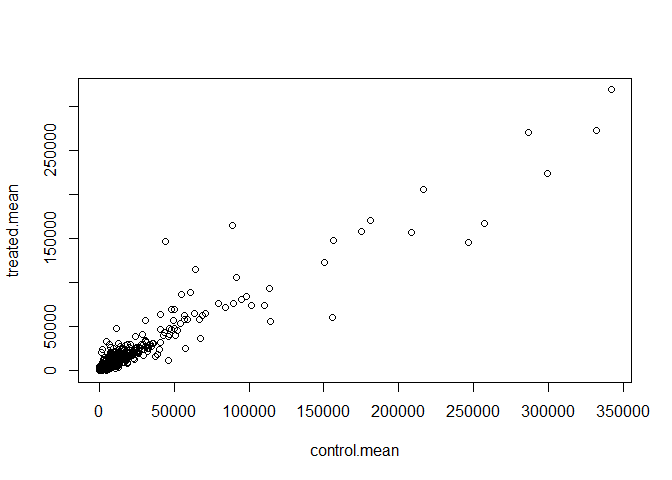
Let’s log transform this count data:
plot(meancounts, log="xy")
Warning in xy.coords(x, y, xlabel, ylabel, log): 15032 x values <= 0 omitted
from logarithmic plot

Warning in xy.coords(x, y, xlabel, ylabel, log): 15281 y values <= 0 omitted
from logarithmic plot
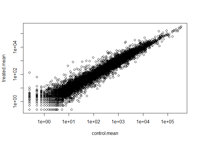
N.B. We most often use log2 for this type of data as it makes the interpretation much more straightforward.
Treated/Control is often called “fold-change”
If there was no change we would have a log2-fc of zero:
log2(10/10)
[1] 0
If we had double the amount of transcript around we would have a log2-fc of one:
log2(20/10)
[1] 1
If we had half as much transcript around we would have a log2-fc of -1
log2(5/10)
[1] -1
Q. Calculate a log2 fold change value for all our genes and add it as a new column to our
meancountsobject.
meancounts$log2f <- log2(meancounts$treated.mean/meancounts$control.mean)


head(meancounts)
                control.mean treated.mean       log2f
ENSG00000000003       900.75       658.00 -0.45303916
ENSG00000000005         0.00         0.00         NaN
ENSG00000000419       520.50       546.00  0.06900279
ENSG00000000457       339.75       316.50 -0.10226805
ENSG00000000460        97.25        78.75 -0.30441833
ENSG00000000938         0.75         0.00        -Inf
log2(40/10)
[1] 2
There are some “funky” log2fc values (NaN and -Inf) here that come about when ever we have 0 mean count values. Typically we would remove these genes from any further analysis - as we can’t say anything about them if we have no data for them.
DESeq analysis
Let’s do this analysis with an estimate of statistical significance using the DESeq2 package.
library(DESeq2)
DESeq (like many bioconductor packages) want it’s input data in a very specific way.
dds <- DESeqDataSetFromMatrix(countData = counts,
                       colData=metadata,
                       design= ~dex)
converting counts to integer mode

Warning in DESeqDataSet(se, design = design, ignoreRank): some variables in
design formula are characters, converting to factors
Run the DESeq analysis pipeline
The main function DESeq()
dds <- DESeq(dds)
estimating size factors

estimating dispersions

gene-wise dispersion estimates

mean-dispersion relationship

final dispersion estimates

fitting model and testing
res <- results(dds)
head(res)
log2 fold change (MLE): dex treated vs control
Wald test p-value: dex treated vs control
DataFrame with 6 rows and 6 columns
                  baseMean log2FoldChange     lfcSE      stat    pvalue
                 <numeric>      <numeric> <numeric> <numeric> <numeric>
ENSG00000000003 747.194195     -0.3507030  0.168246 -2.084470 0.0371175
ENSG00000000005   0.000000             NA        NA        NA        NA
ENSG00000000419 520.134160      0.2061078  0.101059  2.039475 0.0414026
ENSG00000000457 322.664844      0.0245269  0.145145  0.168982 0.8658106
ENSG00000000460  87.682625     -0.1471420  0.257007 -0.572521 0.5669691
ENSG00000000938   0.319167     -1.7322890  3.493601 -0.495846 0.6200029
                     padj
                <numeric>
ENSG00000000003  0.163035
ENSG00000000005        NA
ENSG00000000419  0.176032
ENSG00000000457  0.961694
ENSG00000000460  0.815849
ENSG00000000938        NA
36000* 0.05
[1] 1800
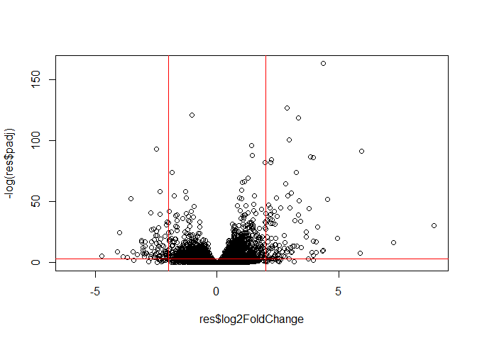
Volcano Plot
This is a main summary results figure from these kinds of studies. It is a plot of Log2-fold-change vs (Adjusted) P-value.
plot(res$log2FoldChange,
     res$padj)
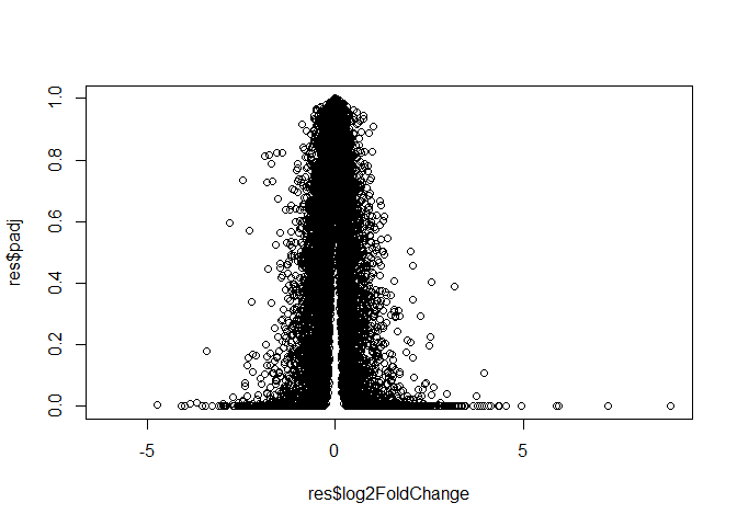
Again this y-axis is highly needs log transforming and we can flip the y-axis with a minus sign so it looks like every other volcano plot.
plot(res$log2FoldChange,
     -log(res$padj))
abline(v=-2, col="red")
abline(v=+2, col="red")
abline(h=-log(0.05), col="red")
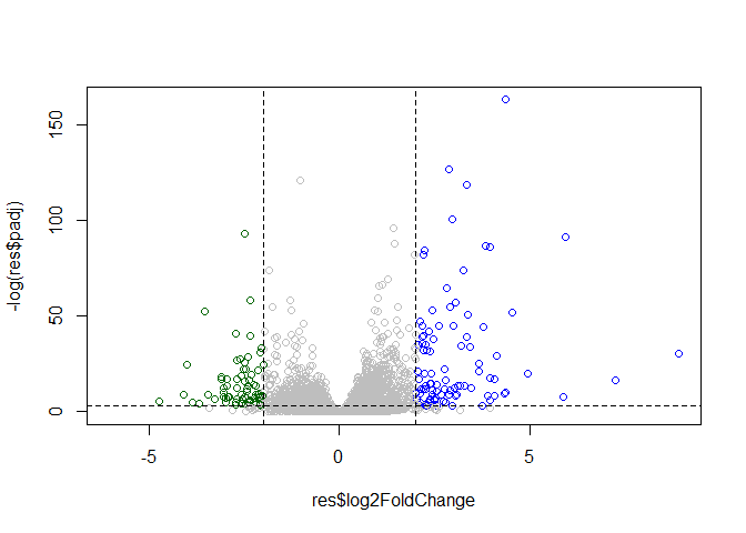
Adding some color annotation
Start with a default base color “gray”
#custom colors
mycols <- rep("gray", nrow(res))
mycols[res$log2FoldChange > 2] <- "blue"
mycols[res$log2FoldChange < -2] <- "darkgreen"
mycols[res$padj >= 0.05 ] <- "gray"

#volcano plot
plot(res$log2FoldChange,
     -log(res$padj),
     col=mycols)

#cut-off dashed lines
abline(v=c(-2,+2), lty=2)
abline(h=-log(0.05), lty=2)
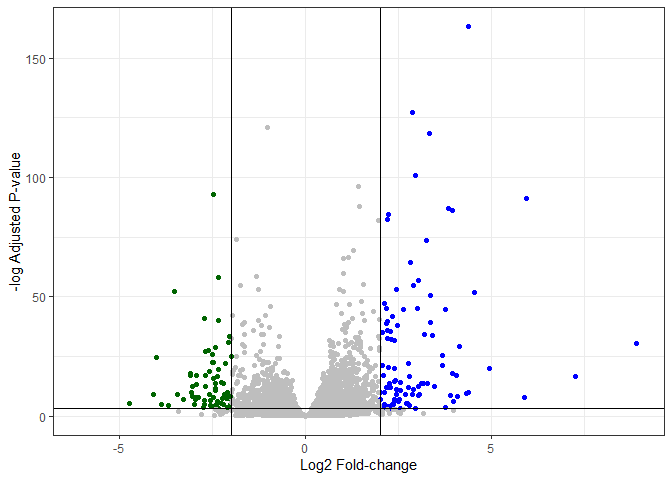
Q. Make a presentation quality ggplot version of this plot. Include cleaer axis labels, a clean theme, you custom colors, cut-off lines and a plot title.
library(ggplot2)

ggplot(res)+
  aes(log2FoldChange,
      -log(padj)
      )+
  geom_point(col=mycols)+
  labs(x="Log2 Fold-change",
       y="-log Adjusted P-value")+
  theme_bw() +
  geom_vline(xintercept=c(-2,2))+
  geom_hline(yintercept=-log(0.05))
Warning: Removed 23549 rows containing missing values or values outside the scale range
(`geom_point()`).
Save our results
Write a CSV file
write.csv(res, file="results.csv")
Add annotation data
We need to add missing annotation data to our main res results object.
This includes the common gene “symbol”
head(res)
log2 fold change (MLE): dex treated vs control
Wald test p-value: dex treated vs control
DataFrame with 6 rows and 6 columns
                  baseMean log2FoldChange     lfcSE      stat    pvalue
                 <numeric>      <numeric> <numeric> <numeric> <numeric>
ENSG00000000003 747.194195     -0.3507030  0.168246 -2.084470 0.0371175
ENSG00000000005   0.000000             NA        NA        NA        NA
ENSG00000000419 520.134160      0.2061078  0.101059  2.039475 0.0414026
ENSG00000000457 322.664844      0.0245269  0.145145  0.168982 0.8658106
ENSG00000000460  87.682625     -0.1471420  0.257007 -0.572521 0.5669691
ENSG00000000938   0.319167     -1.7322890  3.493601 -0.495846 0.6200029
                     padj
                <numeric>
ENSG00000000003  0.163035
ENSG00000000005        NA
ENSG00000000419  0.176032
ENSG00000000457  0.961694
ENSG00000000460  0.815849
ENSG00000000938        NA
We will use R and bioconductor to do this “ID mapping”
library("AnnotationDbi")
library("org.Hs.eg.db")
Let’s see what database we can use for translation/mapping
columns(org.Hs.eg.db)
 [1] "ACCNUM"       "ALIAS"        "ENSEMBL"      "ENSEMBLPROT"  "ENSEMBLTRANS"
 [6] "ENTREZID"     "ENZYME"       "EVIDENCE"     "EVIDENCEALL"  "GENENAME"
[11] "GENETYPE"     "GO"           "GOALL"        "IPI"          "MAP"
[16] "OMIM"         "ONTOLOGY"     "ONTOLOGYALL"  "PATH"         "PFAM"
[21] "PMID"         "PROSITE"      "REFSEQ"       "SYMBOL"       "UCSCKG"
[26] "UNIPROT"
We can use the mapIds()function now to “translate” between any of
these databases.
res$symbol <- mapIds(org.Hs.eg.db,
                     keys=row.names(res), # Our genenames
                     keytype="ENSEMBL",        # Their format
                     column="SYMBOL"          # Format we want
                     )
'select()' returned 1:many mapping between keys and columns
Q. Also add “ENTREZID”, “GENENAME”
res$entrez <- mapIds(org.Hs.eg.db,
                     keys=row.names(res),
                     keytype="ENSEMBL",
                     column="ENTREZID"
                     )
'select()' returned 1:many mapping between keys and columns
res$gename <- mapIds(org.Hs.eg.db,
                     keys=row.names(res),
                     keytype="ENSEMBL",
                     column="GENENAME"
                     )
'select()' returned 1:many mapping between keys and columns
head(res)
log2 fold change (MLE): dex treated vs control
Wald test p-value: dex treated vs control
DataFrame with 6 rows and 9 columns
                  baseMean log2FoldChange     lfcSE      stat    pvalue
                 <numeric>      <numeric> <numeric> <numeric> <numeric>
ENSG00000000003 747.194195     -0.3507030  0.168246 -2.084470 0.0371175
ENSG00000000005   0.000000             NA        NA        NA        NA
ENSG00000000419 520.134160      0.2061078  0.101059  2.039475 0.0414026
ENSG00000000457 322.664844      0.0245269  0.145145  0.168982 0.8658106
ENSG00000000460  87.682625     -0.1471420  0.257007 -0.572521 0.5669691
ENSG00000000938   0.319167     -1.7322890  3.493601 -0.495846 0.6200029
                     padj      symbol      entrez                 gename
                <numeric> <character> <character>            <character>
ENSG00000000003  0.163035      TSPAN6        7105          tetraspanin 6
ENSG00000000005        NA        TNMD       64102            tenomodulin
ENSG00000000419  0.176032        DPM1        8813 dolichyl-phosphate m..
ENSG00000000457  0.961694       SCYL3       57147 SCY1 like pseudokina..
ENSG00000000460  0.815849       FIRRM       55732 FIGNL1 interacting r..
ENSG00000000938        NA         FGR        2268 FGR proto-oncogene, ..
Save annotated results to a CSV file
write.csv(res, file="results_annotated.csv")
Pathway analysis
What known biological pathways do our differentially expressed genes overlap with (i.e. play a role in)?
There lot’s of bioconductor packages to do this type of analysis.
We will use one of the oldest called gage along with pathview to render nice pics of the pathways we find.
We can install these with the command:
BiocManager::install( c("pathview", "gage", "gageData") )
library(pathview)
library(gage)
library(gageData)
Have a wee peak what is in gageData
# Examine the first 2 pathways in this kegg set for humans
data(kegg.sets.hs)
head(kegg.sets.hs, 2)
$`hsa00232 Caffeine metabolism`
[1] "10"   "1544" "1548" "1549" "1553" "7498" "9"

$`hsa00983 Drug metabolism - other enzymes`
 [1] "10"     "1066"   "10720"  "10941"  "151531" "1548"   "1549"   "1551"
 [9] "1553"   "1576"   "1577"   "1806"   "1807"   "1890"   "221223" "2990"
[17] "3251"   "3614"   "3615"   "3704"   "51733"  "54490"  "54575"  "54576"
[25] "54577"  "54578"  "54579"  "54600"  "54657"  "54658"  "54659"  "54963"
[33] "574537" "64816"  "7083"   "7084"   "7172"   "7363"   "7364"   "7365"
[41] "7366"   "7367"   "7371"   "7372"   "7378"   "7498"   "79799"  "83549"
[49] "8824"   "8833"   "9"      "978"
The main gage() function that does the work wants a simple vector as
input.
foldchanges <- res$log2FoldChange
names(foldchanges) <- res$symbol
head(foldchanges)
     TSPAN6        TNMD        DPM1       SCYL3       FIRRM         FGR
-0.35070302          NA  0.20610777  0.02452695 -0.14714205 -1.73228897
The KEGG database uses ENTREZ ids so we need to provide these in our input vector for gage:
names(foldchanges) <- res$entrez
Now we can run gage()
# Get the results
keggres = gage(foldchanges, gsets=kegg.sets.hs)
What is in the output object keggres
attributes(keggres)
$names
[1] "greater" "less"    "stats"
# Look at the first three down (less) pathways
head(keggres$less, 3)
p.geomean stat.mean p.val
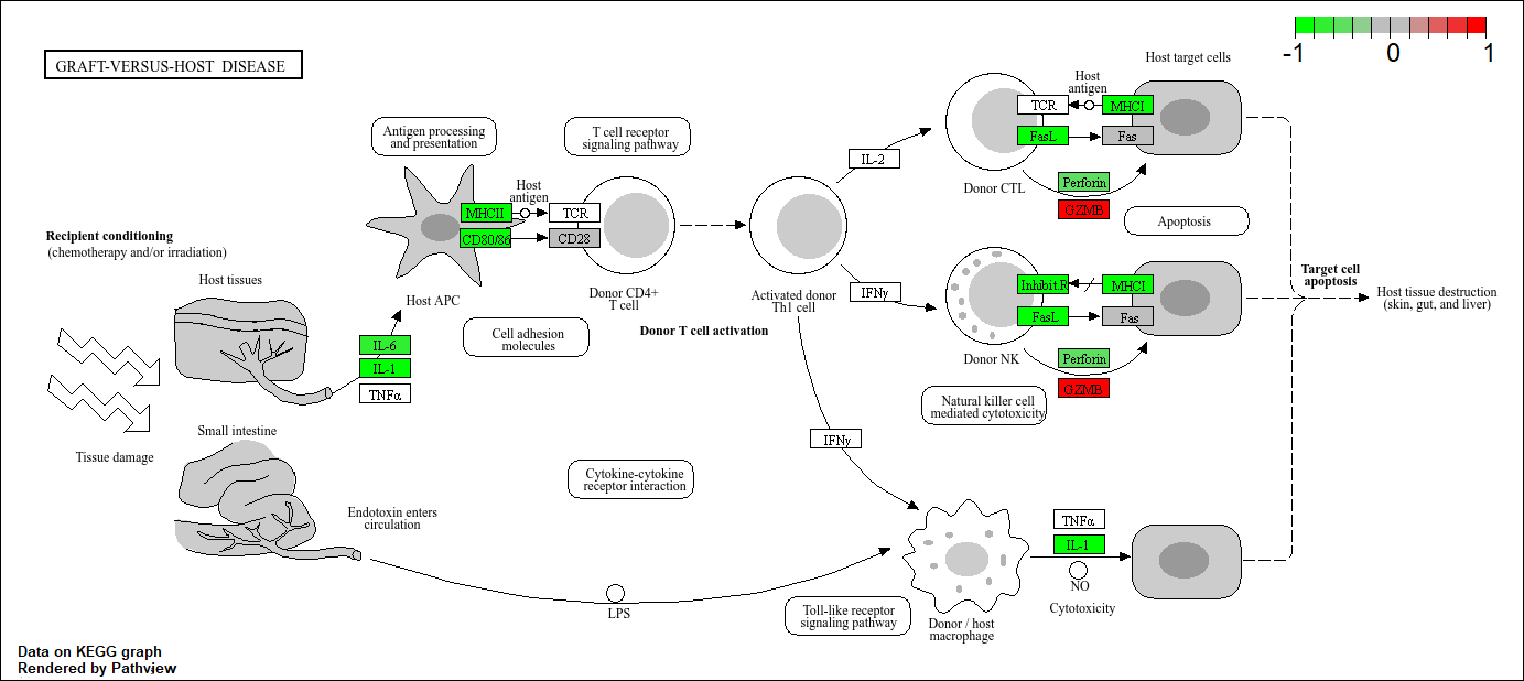
hsa05332 Graft-versus-host disease 0.0004250461 -3.473346 0.0004250461
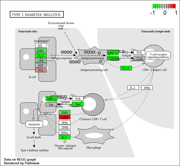
hsa04940 Type I diabetes mellitus 0.0017820293 -3.002352 0.0017820293
hsa05310 Asthma 0.0020045888 -3.009050 0.0020045888
q.val set.size exp1
hsa05332 Graft-versus-host disease 0.09053483 40 0.0004250461
hsa04940 Type I diabetes mellitus 0.14232581 42 0.0017820293
hsa05310 Asthma 0.14232581 29 0.0020045888
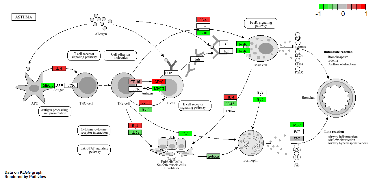
We can use the pathview function to render a figure of any of these pathways along with annotation for our DEGs
Let’s see the hsa05310 Asthma pathway with out DEGs colored up:
pathview(gene.data=foldchanges, pathway.id="hsa05310")
'select()' returned 1:1 mapping between keys and columns

Info: Working in directory C:/Users/josep/OneDrive/BIMM143/bimm143_github/class13

Info: Writing image file hsa05310.pathview.png
Q. Can you render and insert here the pathway figure for “Graft-versus-host disease” and “Type I diabetes”?
Graft Versus host disease
pathview(gene.data=foldchanges, pathway.id="hsa05332")
'select()' returned 1:1 mapping between keys and columns

Info: Working in directory C:/Users/josep/OneDrive/BIMM143/bimm143_github/class13

Info: Writing image file hsa05332.pathview.png
Type I diabetes
pathview(gene.data=foldchanges, pathway.id="hsa04940")
'select()' returned 1:1 mapping between keys and columns

Info: Working in directory C:/Users/josep/OneDrive/BIMM143/bimm143_github/class13

Info: Writing image file hsa04940.pathview.png