Joseph's Site
My classwork for BIMM143
Class 14: RNA-Seq analysis mini-project
Joseph Lo (PID: A18121493)
##Data Import
library(DESeq2)
metaFile <- "GSE37704_metadata.csv"
countFile <- "GSE37704_featurecounts.csv"

# Import metadata and take a peek
colData = read.csv(metaFile, row.names=1)
head(colData)
              condition
SRR493366 control_sirna
SRR493367 control_sirna
SRR493368 control_sirna
SRR493369      hoxa1_kd
SRR493370      hoxa1_kd
SRR493371      hoxa1_kd
# Import countdata
countData = read.csv(countFile, row.names=1)
head(countData)
                length SRR493366 SRR493367 SRR493368 SRR493369 SRR493370
ENSG00000186092    918         0         0         0         0         0
ENSG00000279928    718         0         0         0         0         0
ENSG00000279457   1982        23        28        29        29        28
ENSG00000278566    939         0         0         0         0         0
ENSG00000273547    939         0         0         0         0         0
ENSG00000187634   3214       124       123       205       207       212
                SRR493371
ENSG00000186092         0
ENSG00000279928         0
ENSG00000279457        46
ENSG00000278566         0
ENSG00000273547         0
ENSG00000187634       258
We need to remove the first “length” column from countData to have a
1:1 correspondance with colData rows
Q. Complete the code below to remove the troublesome first column from countData
countData <- countData[,-1]
rownames(colData) == colnames(countData)
[1] TRUE TRUE TRUE TRUE TRUE TRUE
Q. Complete the code below to filter countData to exclude genes (i.e. rows) where we have 0 read count across all samples (i.e. columns).
Remove zero count genes
Some genes (rows) have no count data (i.e. zero values). We should remove these before any further analysis.
to.keep <- rowSums(countData) > 0
countData <- countData[to.keep,]
DESeq Analysis
Setup for DESeq
dds <- DESeqDataSetFromMatrix(countData=countData, colData=colData, design=~condition)
Warning in DESeqDataSet(se, design = design, ignoreRank): some variables in
design formula are characters, converting to factors
Run DESeq
dds <- DESeq(dds)
estimating size factors

estimating dispersions

gene-wise dispersion estimates

mean-dispersion relationship

final dispersion estimates

fitting model and testing
Get Results
res <- results(dds)
#Results
Q. Call the summary() function on your results to get a sense of how many genes are up or down-regulated at the default 0.1 p-value cutoff.
head(res)
log2 fold change (MLE): condition hoxa1 kd vs control sirna
Wald test p-value: condition hoxa1 kd vs control sirna
DataFrame with 6 rows and 6 columns
                 baseMean log2FoldChange     lfcSE       stat      pvalue
                <numeric>      <numeric> <numeric>  <numeric>   <numeric>
ENSG00000279457   29.9136      0.1792571 0.3248216   0.551863 5.81042e-01
ENSG00000187634  183.2296      0.4264571 0.1402658   3.040350 2.36304e-03
ENSG00000188976 1651.1881     -0.6927205 0.0548465 -12.630158 1.43990e-36
ENSG00000187961  209.6379      0.7297556 0.1318599   5.534326 3.12428e-08
ENSG00000187583   47.2551      0.0405765 0.2718928   0.149237 8.81366e-01
ENSG00000187642   11.9798      0.5428105 0.5215598   1.040744 2.97994e-01
                       padj
                  <numeric>
ENSG00000279457 6.86555e-01
ENSG00000187634 5.15718e-03
ENSG00000188976 1.76549e-35
ENSG00000187961 1.13413e-07
ENSG00000187583 9.19031e-01
ENSG00000187642 4.03379e-01
Volcano plot
library(ggplot2)

ggplot(res) +
  aes(log2FoldChange,
      -log(padj))+
  geom_point()
Warning: Removed 1237 rows containing missing values or values outside the scale range
(`geom_point()`).
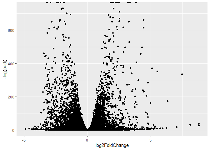
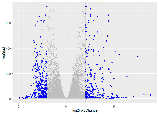
Let’s add some color to this plot along with cutoff lines for fold-change and P-value
Q. Improve this plot by completing the below code, which adds color, axis labels and cutoff lines:
mycols <- rep("gray", nrow(res))
mycols[abs(res$log2FoldChange) > 2] <- "blue"
mycols[res$padj > 0.01] <- "gray"
ggplot(res) +
  aes(log2FoldChange,
      -log(padj))+
  geom_point(col=mycols) +
  geom_vline(xintercept=c(-2,2)) +
  geom_hline(yintercept=-log(0.01))
Warning: Removed 1237 rows containing missing values or values outside the scale range
(`geom_point()`).
Add Annotation
library("AnnotationDbi")
library("org.Hs.eg.db")
columns(org.Hs.eg.db)
 [1] "ACCNUM"       "ALIAS"        "ENSEMBL"      "ENSEMBLPROT"  "ENSEMBLTRANS"
 [6] "ENTREZID"     "ENZYME"       "EVIDENCE"     "EVIDENCEALL"  "GENENAME"
[11] "GENETYPE"     "GO"           "GOALL"        "IPI"          "MAP"
[16] "OMIM"         "ONTOLOGY"     "ONTOLOGYALL"  "PATH"         "PFAM"
[21] "PMID"         "PROSITE"      "REFSEQ"       "SYMBOL"       "UCSCKG"
[26] "UNIPROT"
MapIds
Q. Use the mapIDs() function multiple times to add SYMBOL, ENTREZID and GENENAME annotation to our results by completing the code below.
res$symbol = mapIds(org.Hs.eg.db,
                    keys=rownames(res),
                    keytype="ENSEMBL",
                    column="SYMBOL",
                    multiVals="first")
'select()' returned 1:many mapping between keys and columns
res$entrez = mapIds(org.Hs.eg.db,
                    keys=rownames(res),
                    keytype="ENSEMBL",
                    column="ENTREZID",
                    multiVals="first")
'select()' returned 1:many mapping between keys and columns
res$name =   mapIds(org.Hs.eg.db,
                    keys=row.names(res),
                    keytype="ENSEMBL",
                    column="GENENAME",
                    multiVals="first")
'select()' returned 1:many mapping between keys and columns
head(res, 10)
log2 fold change (MLE): condition hoxa1 kd vs control sirna
Wald test p-value: condition hoxa1 kd vs control sirna
DataFrame with 10 rows and 9 columns
                   baseMean log2FoldChange     lfcSE       stat      pvalue
                  <numeric>      <numeric> <numeric>  <numeric>   <numeric>
ENSG00000279457   29.913579      0.1792571 0.3248216   0.551863 5.81042e-01
ENSG00000187634  183.229650      0.4264571 0.1402658   3.040350 2.36304e-03
ENSG00000188976 1651.188076     -0.6927205 0.0548465 -12.630158 1.43990e-36
ENSG00000187961  209.637938      0.7297556 0.1318599   5.534326 3.12428e-08
ENSG00000187583   47.255123      0.0405765 0.2718928   0.149237 8.81366e-01
ENSG00000187642   11.979750      0.5428105 0.5215598   1.040744 2.97994e-01
ENSG00000188290  108.922128      2.0570638 0.1969053  10.446970 1.51282e-25
ENSG00000187608  350.716868      0.2573837 0.1027266   2.505522 1.22271e-02
ENSG00000188157 9128.439422      0.3899088 0.0467163   8.346304 7.04321e-17
ENSG00000237330    0.158192      0.7859552 4.0804729   0.192614 8.47261e-01
                       padj      symbol      entrez                   name
                  <numeric> <character> <character>            <character>
ENSG00000279457 6.86555e-01          NA          NA                     NA
ENSG00000187634 5.15718e-03      SAMD11      148398 sterile alpha motif ..
ENSG00000188976 1.76549e-35       NOC2L       26155 NOC2 like nucleolar ..
ENSG00000187961 1.13413e-07      KLHL17      339451 kelch like family me..
ENSG00000187583 9.19031e-01     PLEKHN1       84069 pleckstrin homology ..
ENSG00000187642 4.03379e-01       PERM1       84808 PPARGC1 and ESRR ind..
ENSG00000188290 1.30538e-24        HES4       57801 hes family bHLH tran..
ENSG00000187608 2.37452e-02       ISG15        9636 ISG15 ubiquitin like..
ENSG00000188157 4.21963e-16        AGRN      375790                  agrin
ENSG00000237330          NA      RNF223      401934 ring finger protein ..
Save annotated results
Q. Finally for this section let’s reorder these results by adjusted p-value and save them to a CSV file in your current project directory.
write.csv(res, file="deseq_results.csv")
Pathway Analysis
library(pathview)
library(gage)
library(gageData)
data(kegg.sets.hs)
foldchanges <- res$log2FoldChange
names(foldchanges) <- res$entrez
keggres <- gage(foldchanges, gsets=kegg.sets.hs)
# Look at the first few down (less) pathways
head(keggres$less)
                                                  p.geomean stat.mean
hsa04110 Cell cycle                            8.995727e-06 -4.378644
hsa03030 DNA replication                       9.424076e-05 -3.951803
hsa05130 Pathogenic Escherichia coli infection 1.405864e-04 -3.765330
hsa03013 RNA transport                         1.246882e-03 -3.059466
hsa03440 Homologous recombination              3.066756e-03 -2.852899
hsa04114 Oocyte meiosis                        3.784520e-03 -2.698128
                                                      p.val       q.val
hsa04110 Cell cycle                            8.995727e-06 0.001889103
hsa03030 DNA replication                       9.424076e-05 0.009841047
hsa05130 Pathogenic Escherichia coli infection 1.405864e-04 0.009841047
hsa03013 RNA transport                         1.246882e-03 0.065461279
hsa03440 Homologous recombination              3.066756e-03 0.128803765
hsa04114 Oocyte meiosis                        3.784520e-03 0.132458191
                                               set.size         exp1
hsa04110 Cell cycle                                 121 8.995727e-06
hsa03030 DNA replication                             36 9.424076e-05
hsa05130 Pathogenic Escherichia coli infection       53 1.405864e-04
hsa03013 RNA transport                              144 1.246882e-03
hsa03440 Homologous recombination                    28 3.066756e-03
hsa04114 Oocyte meiosis                             102 3.784520e-03
pathview(gene.data=foldchanges, pathway.id="hsa04110")
'select()' returned 1:1 mapping between keys and columns

Info: Working in directory C:/Users/josep/OneDrive/BIMM143/bimm143_github/class14

Info: Writing image file hsa04110.pathview.png
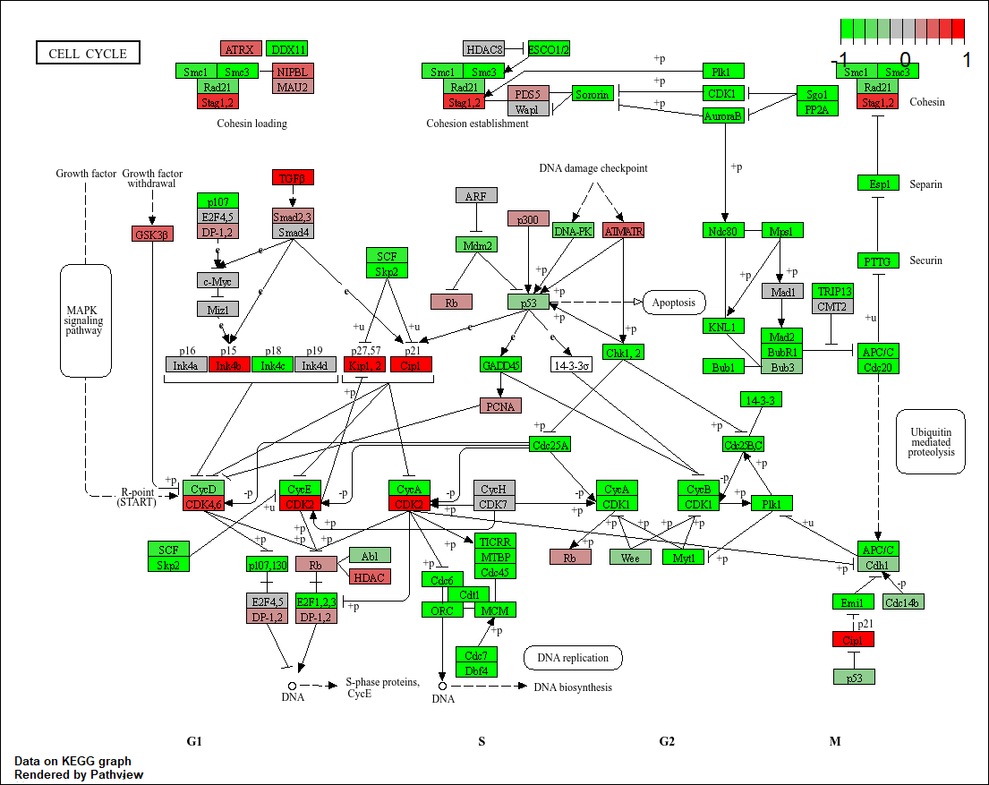
Q. Can you do the same procedure as above to plot the pathview figures for the top 5 down-regulated pathways?
# A different PDF based output of the same data
pathview(gene.data=foldchanges, pathway.id="hsa04110", kegg.native=FALSE)
'select()' returned 1:1 mapping between keys and columns

Warning: reconcile groups sharing member nodes!

     [,1] [,2]
[1,] "9"  "300"
[2,] "9"  "306"

Info: Working in directory C:/Users/josep/OneDrive/BIMM143/bimm143_github/class14

Info: Writing image file hsa04110.pathview.pdf
## Focus on top 5 upregulated pathways here for demo purposes only
keggrespathways <- rownames(keggres$greater)[1:5]

# Extract the 8 character long IDs part of each string
keggresids = substr(keggrespathways, start=1, stop=8)
keggresids
[1] "hsa04060" "hsa05323" "hsa05146" "hsa05332" "hsa04640"
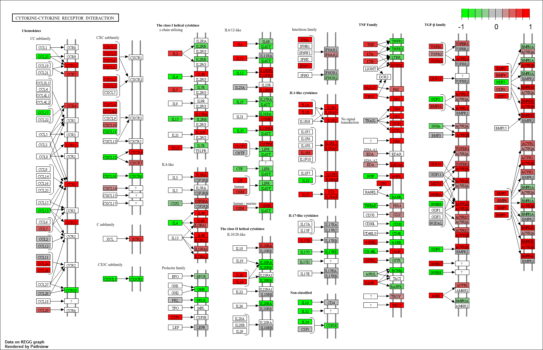
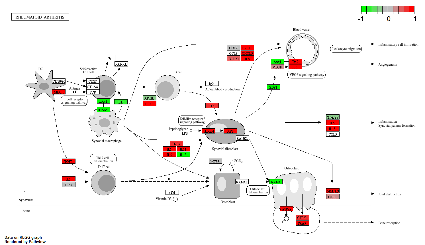
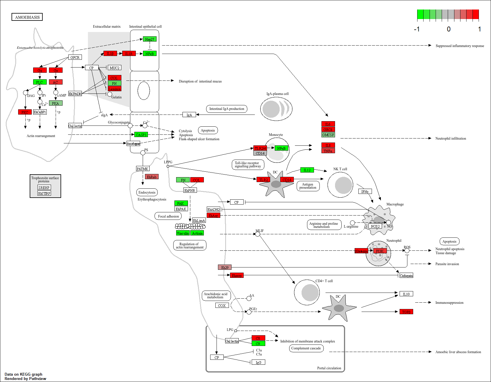
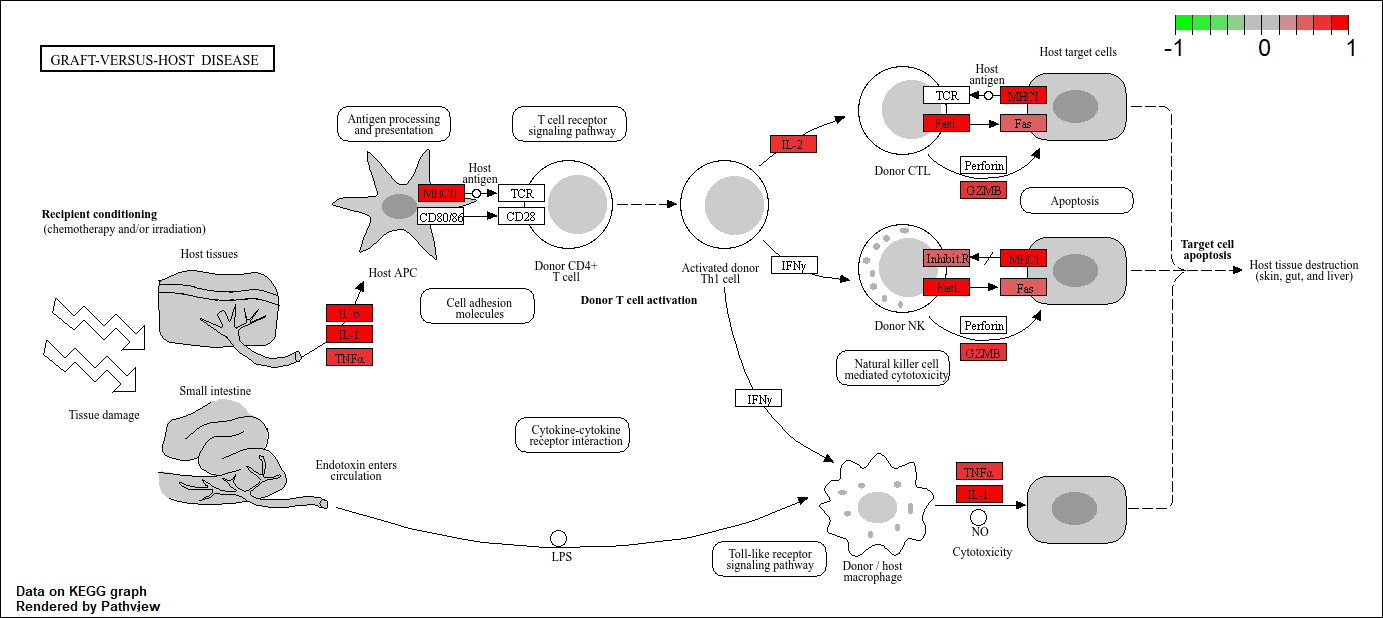
pathview(gene.data=foldchanges, pathway.id=keggresids, species="hsa")
'select()' returned 1:1 mapping between keys and columns

Info: Working in directory C:/Users/josep/OneDrive/BIMM143/bimm143_github/class14

Info: Writing image file hsa04060.pathview.png

'select()' returned 1:1 mapping between keys and columns

Info: Working in directory C:/Users/josep/OneDrive/BIMM143/bimm143_github/class14

Info: Writing image file hsa05323.pathview.png

'select()' returned 1:1 mapping between keys and columns

Info: Working in directory C:/Users/josep/OneDrive/BIMM143/bimm143_github/class14

Info: Writing image file hsa05146.pathview.png

'select()' returned 1:1 mapping between keys and columns

Info: Working in directory C:/Users/josep/OneDrive/BIMM143/bimm143_github/class14

Info: Writing image file hsa05332.pathview.png

'select()' returned 1:1 mapping between keys and columns

Info: Working in directory C:/Users/josep/OneDrive/BIMM143/bimm143_github/class14

Info: Writing image file hsa04640.pathview.png
GO analysis
Focus on the Biological Process “BP” section of GO
data(go.sets.hs)
data(go.subs.hs)

# Focus on Biological Process subset of GO
gobpsets = go.sets.hs[go.subs.hs$BP]
gobpres <-  gage(foldchanges, gsets=gobpsets)
lapply(gobpres, head)
$greater
                                             p.geomean stat.mean        p.val
GO:0007156 homophilic cell adhesion       8.519724e-05  3.824205 8.519724e-05
GO:0002009 morphogenesis of an epithelium 1.396681e-04  3.653886 1.396681e-04
GO:0048729 tissue morphogenesis           1.432451e-04  3.643242 1.432451e-04
GO:0007610 behavior                       1.925222e-04  3.565432 1.925222e-04
GO:0060562 epithelial tube morphogenesis  5.932837e-04  3.261376 5.932837e-04
GO:0035295 tube development               5.953254e-04  3.253665 5.953254e-04
                                              q.val set.size         exp1
GO:0007156 homophilic cell adhesion       0.1951953      113 8.519724e-05
GO:0002009 morphogenesis of an epithelium 0.1951953      339 1.396681e-04
GO:0048729 tissue morphogenesis           0.1951953      424 1.432451e-04
GO:0007610 behavior                       0.1967577      426 1.925222e-04
GO:0060562 epithelial tube morphogenesis  0.3565320      257 5.932837e-04
GO:0035295 tube development               0.3565320      391 5.953254e-04

$less
                                            p.geomean stat.mean        p.val
GO:0048285 organelle fission             1.536227e-15 -8.063910 1.536227e-15
GO:0000280 nuclear division              4.286961e-15 -7.939217 4.286961e-15
GO:0007067 mitosis                       4.286961e-15 -7.939217 4.286961e-15
GO:0000087 M phase of mitotic cell cycle 1.169934e-14 -7.797496 1.169934e-14
GO:0007059 chromosome segregation        2.028624e-11 -6.878340 2.028624e-11
GO:0000236 mitotic prometaphase          1.729553e-10 -6.695966 1.729553e-10
                                                q.val set.size         exp1
GO:0048285 organelle fission             5.841698e-12      376 1.536227e-15
GO:0000280 nuclear division              5.841698e-12      352 4.286961e-15
GO:0007067 mitosis                       5.841698e-12      352 4.286961e-15
GO:0000087 M phase of mitotic cell cycle 1.195672e-11      362 1.169934e-14
GO:0007059 chromosome segregation        1.658603e-08      142 2.028624e-11
GO:0000236 mitotic prometaphase          1.178402e-07       84 1.729553e-10

$stats
                                          stat.mean     exp1
GO:0007156 homophilic cell adhesion        3.824205 3.824205
GO:0002009 morphogenesis of an epithelium  3.653886 3.653886
GO:0048729 tissue morphogenesis            3.643242 3.643242
GO:0007610 behavior                        3.565432 3.565432
GO:0060562 epithelial tube morphogenesis   3.261376 3.261376
GO:0035295 tube development                3.253665 3.253665
Reactome Analysis
We can use the new(ish) Reactome pathway viewer online at https://reactome.org/user/guide
sig_genes <- res[res$padj <= 0.05 & !is.na(res$padj), "symbol"]
print(paste("Total number of significant genes:", length(sig_genes)))
[1] "Total number of significant genes: 8147"
THe website wants a list of genes to work with. We can write one out
with the write.table() function:
write.table(sig_genes, file="significant_genes.txt", row.names=FALSE, col.names=FALSE, quote=FALSE)
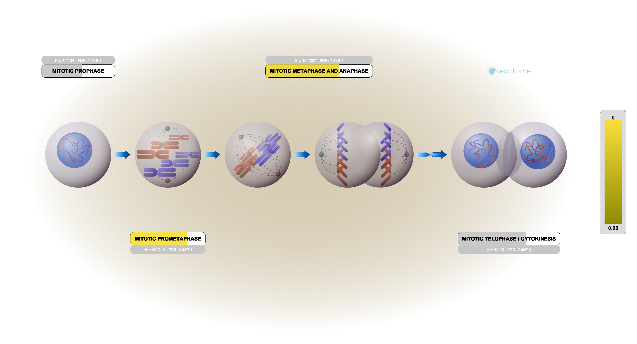
Q: What pathway has the most significant “Entities p-value”? Do the most significant pathways listed match your previous KEGG results? What factors could cause differences between the two methods?
For my data, the Cell Cycle, Mitotic has the most significant entities p-value. This was different than the KEGG results because the KEGG only shows the general process while the Reactome shows the more specific role of how its Mitotic.
And a figure from Reactome: